Implementing Vision Transformer (ViT) from Scratch

Vision Transformer (ViT) is an adaptation of Transformer models to computer vision tasks. It was proposed by Google researchers in 2020 and has since gained popularity due to its impressive performance on various image classification benchmarks. ViT has been shown to achieve state-of-the-art performance on several computer vision tasks and has sparked a lot of interest in the computer vision community.

In this post, we’re going to implement ViT from scratch for image classification using PyTorch. We will also train our model on the CIFAR-10 dataset, a popular benchmark for image classification. By the end of this post, you should have a good understanding of how ViT works and how to use it for your own computer vision projects.

The code for the implementation can be found in this repo.

Overview of the ViT Architecture

ViT’s architecture is inspired by BERT, an encoder-only transformer model that is often used in NLP supervised learning tasks like text classification or named entity recognition. The main idea behind ViT is that an image can be seen as a series of patches, which can be treated as tokens in NLP tasks.

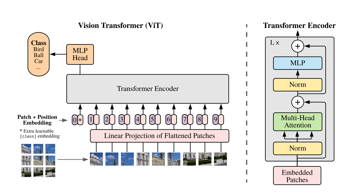
The input image is split into small patches, which are then flattened into sequences of vectors. These vectors are then processed by a transformer encoder, which allows the model to learn interactions between patches through self-attention mechanism. The output of the transformer encoder is then fed into a classification layer that outputs the predicted class of the input image.

In the following sections, we will go through each component of the model and implement it using PyTorch. This will help us understand how ViT models work and how they can be applied to computer vision tasks.

Transform Images into Embeddings

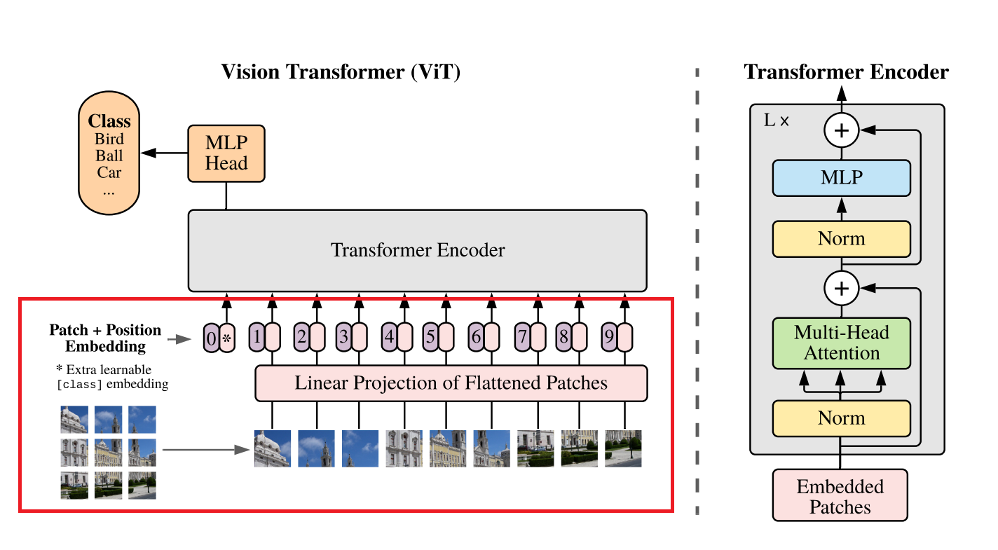
In order to feed input images to a Transformer model, we need to convert the images to a sequence of vectors. This is done by splitting the image into a grid of non-overlapping patches, which are then linearly projected to obtain a fixed-size embedding vector for each patch. We can use PyTorch’s nn.Conv2d layer for this purpose:

class PatchEmbeddings(nn.Module):
    """
    Convert the image into patches and then project them into a vector space.
    """

    def __init__(self, config):
        super().__init__()
        self.image_size = config["image_size"]
        self.patch_size = config["patch_size"]
        self.num_channels = config["num_channels"]
        self.hidden_size = config["hidden_size"]
        # Calculate the number of patches from the image size and patch size
        self.num_patches = (self.image_size // self.patch_size) ** 2
        # Create a projection layer to convert the image into patches
        # The layer projects each patch into a vector of size hidden_size
        self.projection = nn.Conv2d(self.num_channels, self.hidden_size, kernel_size=self.patch_size, stride=self.patch_size)

    def forward(self, x):
        # (batch_size, num_channels, image_size, image_size) -> (batch_size, num_patches, hidden_size)
        x = self.projection(x)
        x = x.flatten(2).transpose(1, 2)
        return x

kernel_size=self.patch_size and stride=self.patch_size are to make sure the layer’s filter is applied to non-overlapping patches.

After the patches are converted to a sequence of embeddings, the [CLS] token is added to the beginning of the sequence, it will be used later in the classification layer to classify the image. The [CLS] token’s embedding is learned during training.

As patches from different positions may contribute differently to the final predictions, we also need a way to encode patch positions into the sequence. We’re going to use learnable position embeddings to add positional information to the embeddings. This is similar to how position embeddings are used in Transformer models for NLP tasks.

class Embeddings(nn.Module):
    """
    Combine the patch embeddings with the class token and position embeddings.
    """
        
    def __init__(self, config):
        super().__init__()
        self.config = config
        self.patch_embeddings = PatchEmbeddings(config)
        # Create a learnable [CLS] token
        # Similar to BERT, the [CLS] token is added to the beginning of the input sequence
        # and is used to classify the entire sequence
        self.cls_token = nn.Parameter(torch.randn(1, 1, config["hidden_size"]))
        # Create position embeddings for the [CLS] token and the patch embeddings
        # Add 1 to the sequence length for the [CLS] token
        self.position_embeddings = \
            nn.Parameter(torch.randn(1, self.patch_embeddings.num_patches + 1, config["hidden_size"]))
        self.dropout = nn.Dropout(config["hidden_dropout_prob"])

    def forward(self, x):
        x = self.patch_embeddings(x)
        batch_size, _, _ = x.size()
        # Expand the [CLS] token to the batch size
        # (1, 1, hidden_size) -> (batch_size, 1, hidden_size)
        cls_tokens = self.cls_token.expand(batch_size, -1, -1)
        # Concatenate the [CLS] token to the beginning of the input sequence
        # This results in a sequence length of (num_patches + 1)
        x = torch.cat((cls_tokens, x), dim=1)
        x = x + self.position_embeddings
        x = self.dropout(x)
        return x

At this step, the input image is converted to a sequence of embeddings with positional information and ready to be fed into the transformer layer.

Multi-head Attention

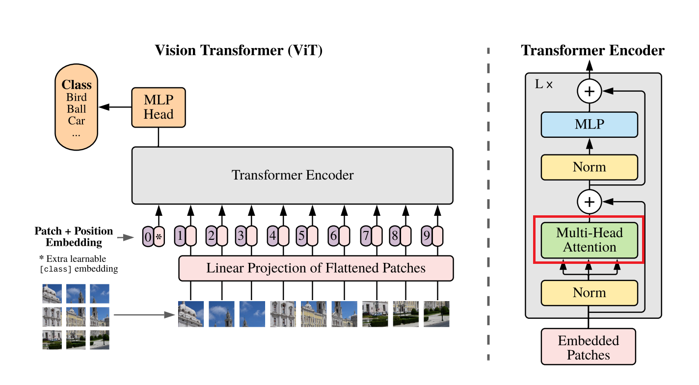
Before going through the transformer encoder, we first explore the multi-head attention module, which is its core component. The multi-head attention is used to compute the interactions between different patches in the input image. The multi-head attention consists of multiple attention heads, each of which is a single attention layer.

Let’s implement a head of the multi-head attention module. The module takes a sequence of embeddings as input and computes query, key, and value vectors for each embedding. The query and key vectors are then used to compute the attention weights for each token. The attention weights are then used to compute new embeddings using a weighted sum of the value vectors. We can think of this mechanism as a soft version of a database query, where the query vectors find the most relevant key vectors in the database, and the value vectors are retrieved to compute the query output.

class AttentionHead(nn.Module):
    """
    A single attention head.
    This module is used in the MultiHeadAttention module.
    """
    def __init__(self, hidden_size, attention_head_size, dropout, bias=True):
        super().__init__()
        self.hidden_size = hidden_size
        self.attention_head_size = attention_head_size
        # Create the query, key, and value projection layers
        self.query = nn.Linear(hidden_size, attention_head_size, bias=bias)
        self.key = nn.Linear(hidden_size, attention_head_size, bias=bias)
        self.value = nn.Linear(hidden_size, attention_head_size, bias=bias)

        self.dropout = nn.Dropout(dropout)
    
    def forward(self, x):
        # Project the input into query, key, and value
        # The same input is used to generate the query, key, and value,
        # so it's usually called self-attention.
        # (batch_size, sequence_length, hidden_size) -> (batch_size, sequence_length, attention_head_size)
        query = self.query(x)
        key = self.key(x)
        value = self.value(x)
        # Calculate the attention scores
        # softmax(Q*K.T/sqrt(head_size))*V
        attention_scores = torch.matmul(query, key.transpose(-1, -2))
        attention_scores = attention_scores / math.sqrt(self.attention_head_size)
        attention_probs = nn.functional.softmax(attention_scores, dim=-1)
        attention_probs = self.dropout(attention_probs)
        # Calculate the attention output
        attention_output = torch.matmul(attention_probs, value)
        return (attention_output, attention_probs)

The outputs from all attention heads are then concatenated and linearly projected to obtain the final output of the multi-head attention module.

class MultiHeadAttention(nn.Module):
    """
    Multi-head attention module.
    This module is used in the TransformerEncoder module.
    """

    def __init__(self, config):
        super().__init__()
        self.hidden_size = config["hidden_size"]
        self.num_attention_heads = config["num_attention_heads"]
        # The attention head size is the hidden size divided by the number of attention heads
        self.attention_head_size = self.hidden_size // self.num_attention_heads
        self.all_head_size = self.num_attention_heads * self.attention_head_size
        # Whether or not to use bias in the query, key, and value projection layers
        self.qkv_bias = config["qkv_bias"]
        # Create a list of attention heads
        self.heads = nn.ModuleList([])
        for _ in range(self.num_attention_heads):
            head = AttentionHead(
                self.hidden_size,
                self.attention_head_size,
                config["attention_probs_dropout_prob"],
                self.qkv_bias
            )
            self.heads.append(head)
        # Create a linear layer to project the attention output back to the hidden size
        # In most cases, all_head_size and hidden_size are the same
        self.output_projection = nn.Linear(self.all_head_size, self.hidden_size)
        self.output_dropout = nn.Dropout(config["hidden_dropout_prob"])

    def forward(self, x, output_attentions=False):
        # Calculate the attention output for each attention head
        attention_outputs = [head(x) for head in self.heads]
        # Concatenate the attention outputs from each attention head
        attention_output = torch.cat([attention_output for attention_output, _ in attention_outputs], dim=-1)
        # Project the concatenated attention output back to the hidden size
        attention_output = self.output_projection(attention_output)
        attention_output = self.output_dropout(attention_output)
        # Return the attention output and the attention probabilities (optional)
        if not output_attentions:
            return (attention_output, None)
        else:
            attention_probs = torch.stack([attention_probs for _, attention_probs in attention_outputs], dim=1)
            return (attention_output, attention_probs)

Transformer Encoder

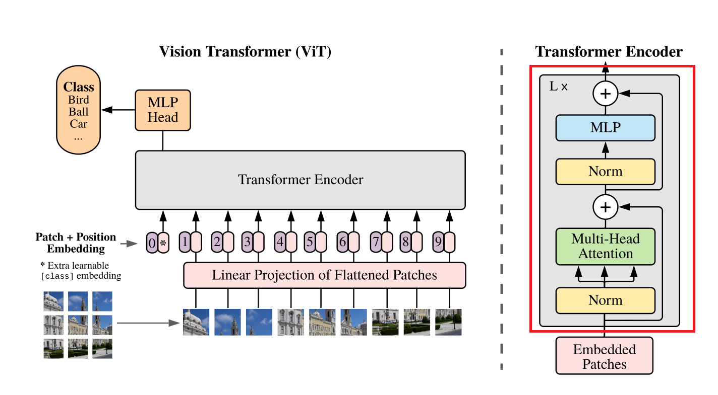
The transformer encoder is made of a stack of transformer layers. Each transformer layer mainly consists of a multi-head attention module that we just implemented and a feed-forward network. To better scale the model and stabilize training, two Layer normalization layers and skip connections are added to the transformer layer.

Let’s implement a transformer layer (referred to as Block in the code as it’s the building block for the transformer encoder). We’ll begin with the feed-forward network, which is a simple two-layer MLP with GELU activation in between.

class MLP(nn.Module):
    """
    A multi-layer perceptron module.
    """

    def __init__(self, config):
        super().__init__()
        self.dense_1 = nn.Linear(config["hidden_size"], config["intermediate_size"])
        self.activation = NewGELUActivation()
        self.dense_2 = nn.Linear(config["intermediate_size"], config["hidden_size"])
        self.dropout = nn.Dropout(config["hidden_dropout_prob"])

    def forward(self, x):
        x = self.dense_1(x)
        x = self.activation(x)
        x = self.dense_2(x)
        x = self.dropout(x)
        return x

We have implemented the multi-head attention and the MLP, we can combine them to create the transformer layer. The skip connections and layer normalization are applied to the input of each layer

class Block(nn.Module):
    """
    A single transformer block.
    """

    def __init__(self, config):
        super().__init__()
        self.attention = MultiHeadAttention(config)
        self.layernorm_1 = nn.LayerNorm(config["hidden_size"])
        self.mlp = MLP(config)
        self.layernorm_2 = nn.LayerNorm(config["hidden_size"])

    def forward(self, x, output_attentions=False):
        # Self-attention
        attention_output, attention_probs = \
            self.attention(self.layernorm_1(x), output_attentions=output_attentions)
        # Skip connection
        x = x + attention_output
        # Feed-forward network
        mlp_output = self.mlp(self.layernorm_2(x))
        # Skip connection
        x = x + mlp_output
        # Return the transformer block's output and the attention probabilities (optional)
        if not output_attentions:
            return (x, None)
        else:
            return (x, attention_probs)

The transformer encoder stacks multiple transformer layers sequentially:

class Encoder(nn.Module):
    """
    The transformer encoder module.
    """

    def __init__(self, config):
        super().__init__()
        # Create a list of transformer blocks
        self.blocks = nn.ModuleList([])
        for _ in range(config["num_hidden_layers"]):
            block = Block(config)
            self.blocks.append(block)

    def forward(self, x, output_attentions=False):
        # Calculate the transformer block's output for each block
        all_attentions = []
        for block in self.blocks:
            x, attention_probs = block(x, output_attentions=output_attentions)
            if output_attentions:
                all_attentions.append(attention_probs)
        # Return the encoder's output and the attention probabilities (optional)
        if not output_attentions:
            return (x, None)
        else:
            return (x, all_attentions)

ViT for image classification

After inputting the image to the embedding layer and transformer encoder, we obtain new embeddings for both the image patches and the [CLS] token. At this point, the embeddings should have some useful signals for classification after being processed by the transformer encoder. Similar to BERT, we’ll use only the [CLS] token’s embedding to pass to the classification layer.

The classification layer is a fully connected layer that takes the [CLS] embedding as input and outputs logits for each image. The following code implements the ViT model for image classification:

class ViTForClassfication(nn.Module):
    """
    The ViT model for classification.
    """

    def __init__(self, config):
        super().__init__()
        self.config = config
        self.image_size = config["image_size"]
        self.hidden_size = config["hidden_size"]
        self.num_classes = config["num_classes"]
        # Create the embedding module
        self.embedding = Embeddings(config)
        # Create the transformer encoder module
        self.encoder = Encoder(config)
        # Create a linear layer to project the encoder's output to the number of classes
        self.classifier = nn.Linear(self.hidden_size, self.num_classes)
        # Initialize the weights
        self.apply(self._init_weights)

    def forward(self, x, output_attentions=False):
        # Calculate the embedding output
        embedding_output = self.embedding(x)
        # Calculate the encoder's output
        encoder_output, all_attentions = self.encoder(embedding_output, output_attentions=output_attentions)
        # Calculate the logits, take the [CLS] token's output as features for classification
        logits = self.classifier(encoder_output[:, 0])
        # Return the logits and the attention probabilities (optional)
        if not output_attentions:
            return (logits, None)
        else:
            return (logits, all_attentions)

To train the model, you can follow the standard steps for training classification models. You can find the training script here.

Results

As The goal is not to achieve state-of-the-art performance but to demonstrate how the model works intuitively, the model I trained is much smaller than the original ViT models described in the paper, which have at least 12 layers and a hidden size of 768. The model config I used for the training is:

{
    "patch_size": 4,
    "hidden_size": 48,
    "num_hidden_layers": 4,
    "num_attention_heads": 4,
    "intermediate_size": 4 * 48,
    "hidden_dropout_prob": 0.0,
    "attention_probs_dropout_prob": 0.0,
    "initializer_range": 0.02,
    "image_size": 32,
    "num_classes": 10,
    "num_channels": 3,
    "qkv_bias": True,
}

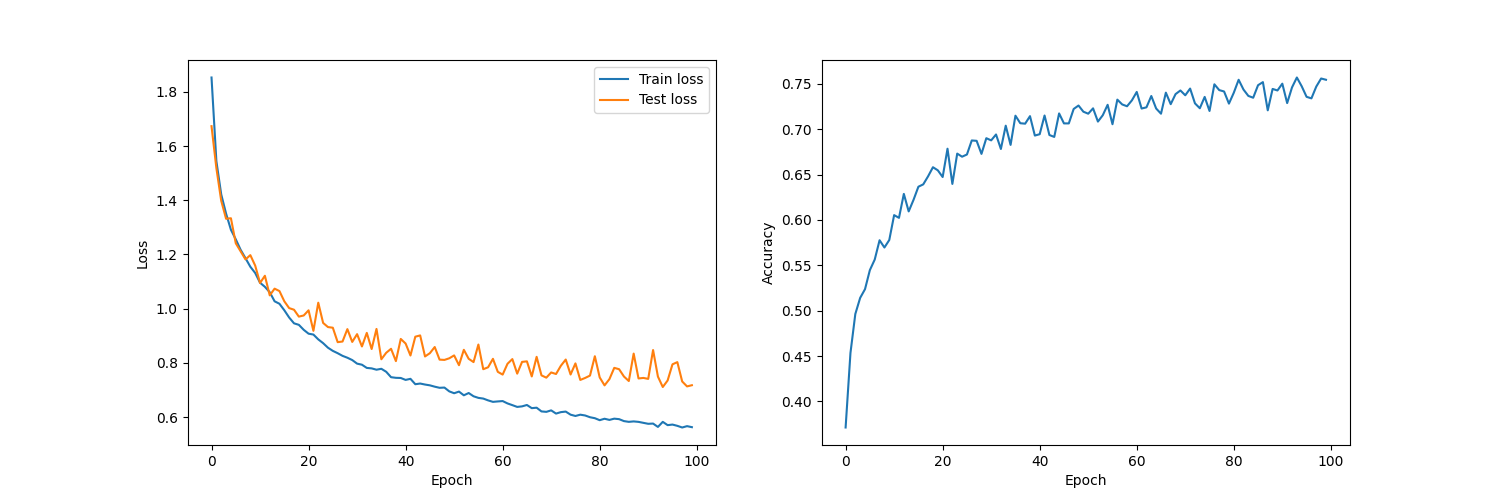
The model is trained on the CIFAR-10 dataset for 100 epochs, with a batch size of 256. The learning rate was set to 0.01, and no learning rate schedule was used. The model is able to achieve 75.5% accuracy after 100 epochs of training. The following shows the training loss, test loss, and accuracy on the test set during training.

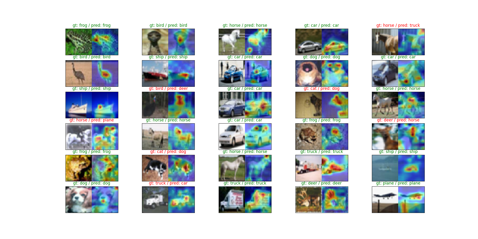
The plot below displays the model’s attention maps to some test images. You can see that the model is able to identify objects from different classes. It learned to focus on the objects and ignore the background.

Conclusion

In this post, we have learned how the Vision Transformer works, from the embedding layer to the transformer encoder and finally to the classification layer. We have also learned how to implement each component of the model using PyTorch.

Since this implementation is not intended for production use, I recommend using more mature libraries for transformers, such as HuggingFace, if you intend to train full-sized models or train them on large datasets.